TecnicaMotori - Racing line

Home Donate Download About Contact Italiano

Racetrack driving: choosing the racing line
© 2017 Mattia Piron. All rights reserved.

Introduction

Computer simulation

A practical method

An example for Adria raceway

Bibliography

SEPTEMBER 15th, 2020

Introduction top

One of the most important factors in improving your lap time is to use the most effective line possible. Even a driver who is capable of taking a vehicle to the limit cannot set record times if he or she misses a braking or apex. The choice of racing line is usually not a problem for a professional driver, but it can be for the amateur. In driving courses (or in tutorials on the internet) the trajectories are often one of the most popular topics, but most of the time they are explained using as an example the classic curves: sharp curve, hairpin and chicane. We talk about "classic" racing line, delayed apex and trail braking. It is also explained that, in a sequence of curves, it is better to sacrifice the racing line in the first curve in order to come out as strong as possible in the last one.

Although all these notions are correct and it is right to know them, it is difficult to translate them into a real track lap. That's because every turn on every circuit is unique, and the ideal racing line depends on both the previous turns and the subsequent ones. So what do you usually do?

We enter the track, following the trajectories that we think are best based on our experience, or copying the trajectories of the strongest drivers. But are we really sure that those trajectories are actually the best ones? Nowadays there are software that, given a circuit and a vehicle, are able to calculate the racing line that allows to obtain the best lap time. The same calculation can be made even without a computer, and without knowing mathematics, we will see later how.

Computer simulation top

Simulations are used a lot by teams to make the basic setup of the vehicle: given the limits imposed on the hours of testing and the maximum number of tires available to each team, a computer simulation allows you to test a huge number of different setups without moving the car (or bike) from the box. However, in addition to performing the setup, the simulations are also used to find the best trajectories, which the pilot will then try to follow.

In strictly mathematical terms, optimizing the racing line means finding the function that, imposed the constraints given by the limits of the track and the physical behavior of the vehicle, allows to minimize the travel time. To find this function have been used and tested several methods, in bibliography are reported some articles on the subject, for those who want to deepen. In particular, the article "Searching for the Optimal Racing Line Using Genetic Algorithms"^[1] proposes a very interesting approach, both for its implementation (which allows you to achieve an excellent result in a short time) and because it lays the groundwork for the "manual" method (or "without computer") described later. Although the article is dedicated to videogames, the simulations were carried out using the open-source driving simulator Torcs. The results are also valid in the real world, because the physics of a driving simulator tries to mimic as correctly as possible that of a real vehicle.

Basically, it says this: the optimal racing line in a given circuit will be a mix between the racing line that minimizes the curvature (the smaller the curvature, the greater will be the average speed and therefore shorter will be the lap time) and the one that minimizes the traveled space (if I do less meters I could take less time). The racing line that minimizes the curvature is nothing but the one that allows to maintain the speed of the vehicle as much as possible. Extremely effective especially with low-power vehicles or with a very narrow range of engine power, for which it is important to lose as little speed as possible and keep the engine always within its optimum rpm.

If we call α_SP the shortest path racing line and α_MCP the minimum curvature one, the best one will be comprised between these two:

α_BEST = α_SP * ε + α_MCP * (1 - ε)

Where ε is the "weight": if ε = 0, then the best racing line is α_MCP, if it is equal to 1 is α_SP, any value between 0 and 1 means that the best path will be a mix of the two. It turns out that, in 9 out of 11 tracks tested, ε = 0. On the two remaining track, ε assumes a small value (0.25 and 0.33), in these cases the best trajectory is a mix between the two, but the one with the least curvature is predominant. Considering a complete lap of the track, we can say that in most cases the best trajectory is the one with the least curvature.

The article then proceeds by dividing the track into sectors, and finding the best trajectory for each sector. No longer is a ε "total" considered, but as many ε as sectors. You find different ε values for each sector, and your lap time improves. In the guided sections it is better to follow the trajectory that minimizes the curvature, to keep the average speed as high as possible, while in the fast sections it is better to travel less road. In fact, in all those stretches where even at full throttle you can follow the shortest path, it is not necessary to lengthen the path by following the one with less curvature.

A practical method top

With a little ingenuity and without a computer, anyone can find the two boundary trajectories described above. Suppose we have a scale model of the track, in which the limits of the track are defined by walls (or nails, or whatever). If we insert a string into this model, and pull on its ends, we have found the trajectory that minimizes the space traveled. In fact, by keeping the string in tension, it shortens as much as it can.

Now, keep in mind that any action in nature follows the path of least energy consumption: as water flows in the direction where there are least losses, a beam bends taking the shape that minimizes elastic energy. The elastic energy of a beam depends on its curvature: the lower the curvature, the lower the elastic energy. Therefore, by inserting any elastic beam into our track model, it will bend into the shape that minimizes curvature. The beam can be a wooden or a steel strip... the important thing is that it always remains in the elastic field: removing the limits of the track, it must automatically become straight.

Now, we have a scale model of the track we will be racing on and the two boundary trajectories. We can photograph them, or copy them on a sheet of paper, and the next time we go to the track we will try to follow them. We can start by following the trajectory that minimizes the curvature and then, lap after lap, "shorten" the road in the fast sections, based on our driving sensations and chronometric feedback.

An example for Adria raceway top

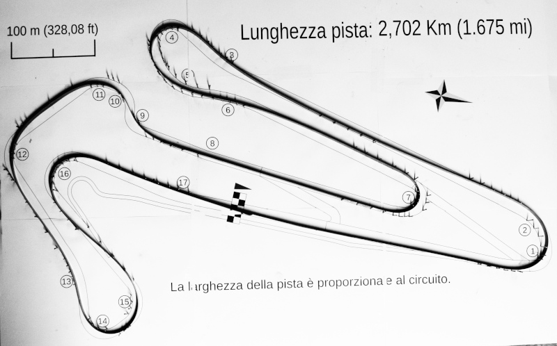
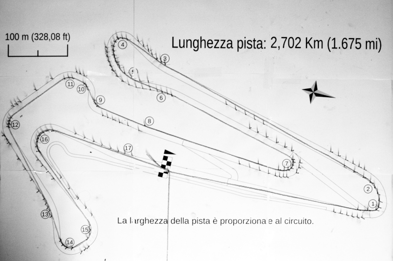
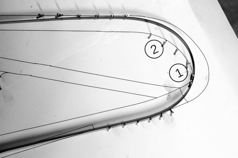
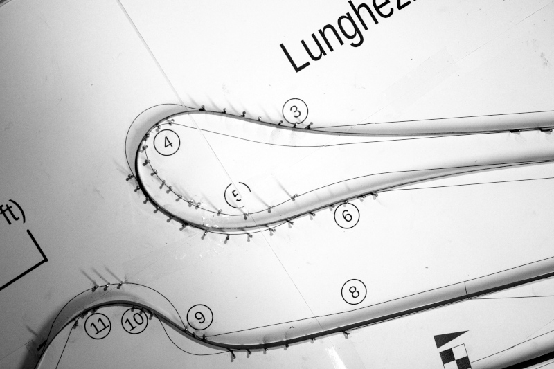
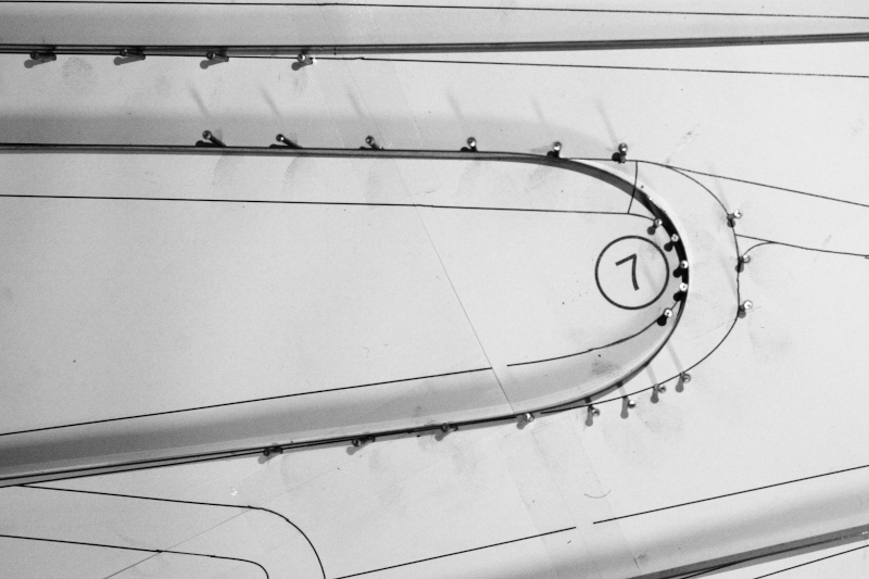
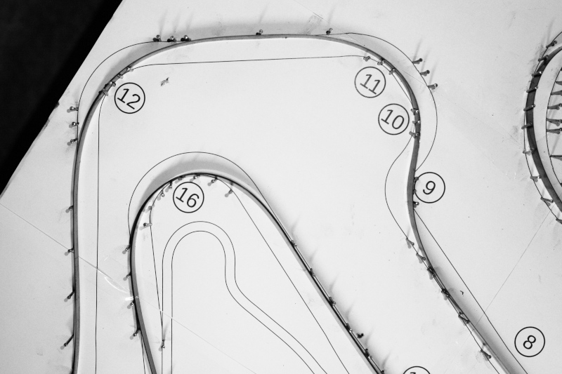
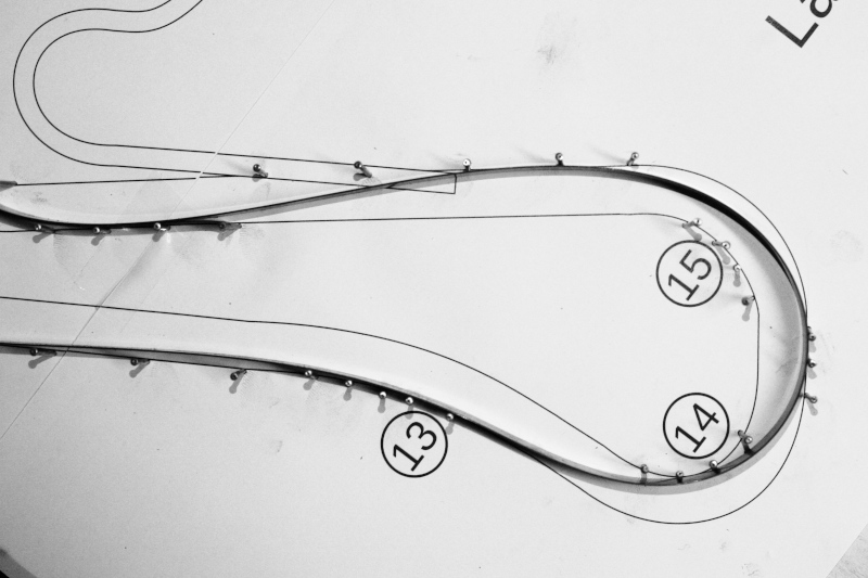
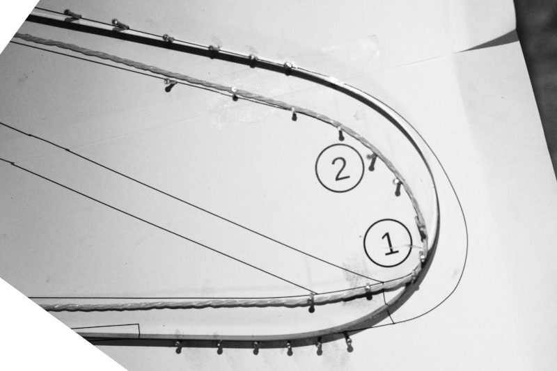
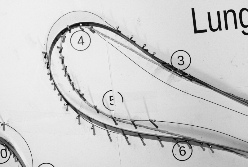
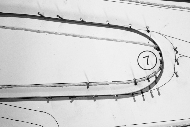
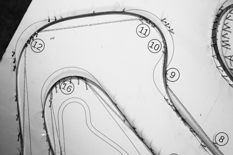
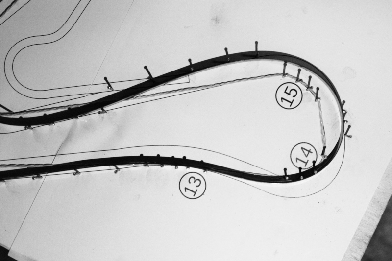
The method described above is illustrated in the following images, using as an example the circuit of Adria, in the province of Rovigo. The image of the circuit was printed on a sheet of about 80x55 cm, glued on a wooden board, and nails were used to delimit the track. To define the trajectory that minimizes the curvature was used a harmonic steel tape 15x0.5mm, soft enough to follow even the tightest curves, but sufficiently elastic not to suffer permanent deformation. Moreover, it could slide on the pegs, adapting itself in the most optimal way to the curves of the circuit.

A common string pulled at the ends was used to define the shortest distance trajectory.

General view of racetrack

Modello della pista con traiettorie

Minimum curvature racing line

Modello della pista con traiettorie

Shortest path racing line

Corner detail

Ingrandimento curve 1-2

Ingrandimento curve 3-4-5-6

Ingrandimento curva 7

Ingrandimento curve 8-9-10-11-12-16

Ingrandimento curve 13-14-15